Exact results for problems at the frontier of quantum computing.
We deliver software solutions to some of the biggest challenges in making quantum computers useful. Our tools provide mathematically exact answers in domains of exponential complexity: How to simulate a quantum computation with classical resources as fast as possible? How to use quantum-HPC resources as efficiently as possible? How to optimally distribute quantum circuits between different QPUs of limited capacity?
Alternative simulation tools are not guaranteed to be close to optimal strategies. Our software (patent filed) is the first to carry out these tasks with performance guarantees - usually beating alternative methods or landing on the mathematical optimum.
Classical simulations

Hybrid quantum computing

Distributed quantum computing
The question of quantum supremacy.
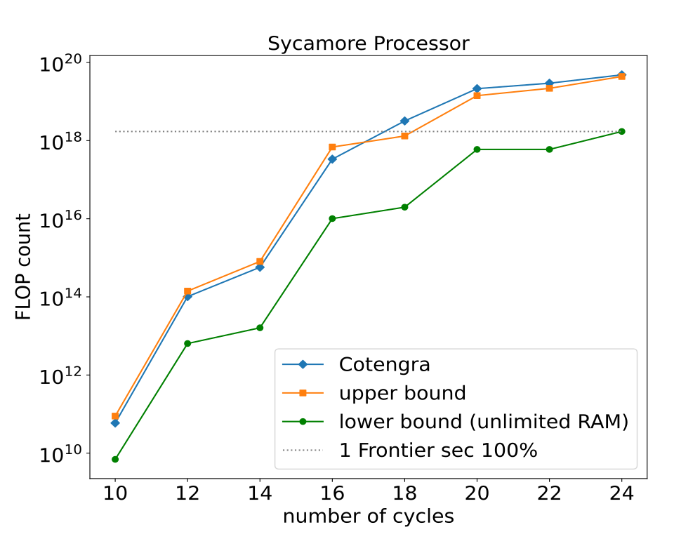
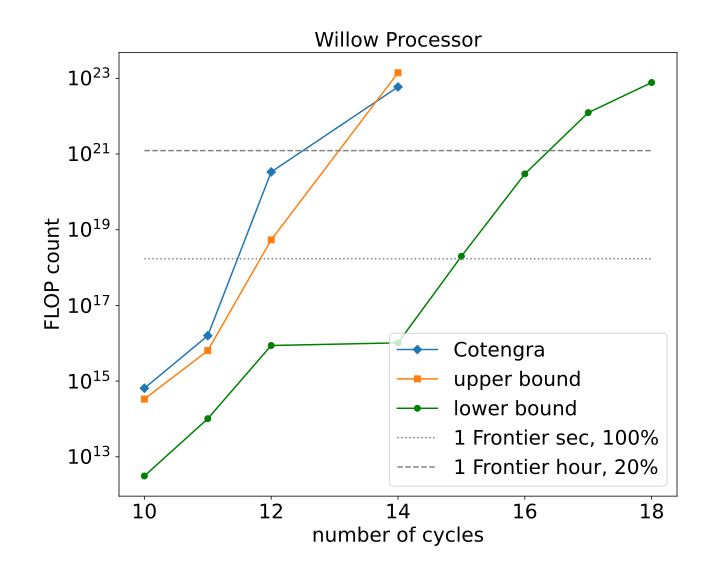
The lower and upper bounds on classical simulation costs provided by our tools can be used to settle questions around quantum supremacy. Specifically, one can bound how many floating point operations (FLOPs) are needed to contract a given quantum circuit exactly. If the lower bound exceeds a given budget (e.g., one second on Frontier, one hour on Frontier), we call the corresponding quantum processor quantum supreme. The two figures below show the lower bound and upper bound obtained using our software for the Google Sycamore processor and their more recent Willow processor as a function of the number of cycles.
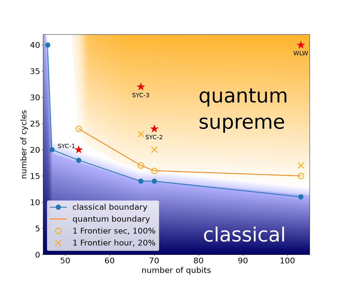
These results can be used to chart the quantum supremacy diagram of superconducting quantum processors of the Sycamore-Willow architecture below. The diagram consists of a provably classically simulable regime, where our upper bound sits below the computational budget of one Frontier second and a quantum supreme regime, where even the lower bound exceeds the designated computational budget, separated by a narrow grey zone. While the set computational budget is arbitrary, redefining it only shifts the quantum supremacy boundary marginally (cf. orange crosses corresponding to one Frontier hour at 20% efficiency). We note that either way, the Willow processor with 40 cycles of operation is located deep in the quantum supremacy regime.